Pylab, R, and QtiPlot Plotting Compared

Today I want to compare and contrast the plotting of statistical graphics in three very neat software packages freely available:

• Pylab via Ipython
• The R Statistical Computing Environment and
• QtiPlot

First we'll take a look at the raw table of numbers to be plotted, I'll show you the resultant plots, and finally I'll show you the code or steps necessary to get to those plots.

---

In the sample dataset above, I've included an "X Axis" column composed of 7 integers simply called X. I've also included two Y columns of means and two columns containing the Standard Errors of the datasets from which those means came. My plotting aim was to create a plot containing two lines describing the two Y columns and error bars matching the values from the two Standard Error columns.

---

Pylab plot





R plot





QtiPlot

---

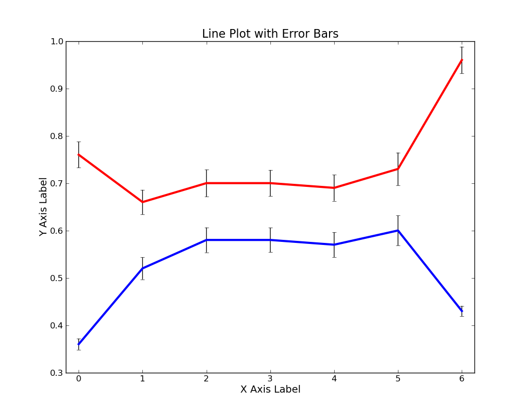
As you can see from the above plots, no one of these three software packages produces a bad looking plot. Some of the graphical parameters (such as font size, type of major axis ticks, whether or not a full box is drawn around the plotting area, and how far the plot title is from the top of the plotting area) are different from program to program, but that's more a matter of my unwillingness to get the programs to output exactly similar graphs than an inability in the programs themselves.



How I got the plots using Pylab and R 
First and foremost is the fact that Pylab and R require you to type in some code to do your plotting whereas QtiPlot gives you a point-and-click GUI interface to complete the task. Pylab and R have their own idiosyncratic syntax for plotting, but thankfully neither requires much more code than the other. If you didn't know already, Pylab is a module of python and therefore allows you to seamlessly weave plotting commands into pure python code. It will therefore be advantageous for anyone who already has a Python background to use Pylab. Below I will show you the code I used to make the plots.

Pylab via IPython

1. infile = open('/home/inkhorn/Documents/data.csv','rb')
2. data = loadtxt(infile, delimiter=',')
3. errorbar(data[:,0], data[:,1], yerr=data[:,2],color='b',ecolor='k',elinewidth=1,linewidth=3);
4. errorbar(data[:,0], data[:,3], yerr=data[:,4],color='r',ecolor='k',elinewidth=1,linewidth=3);
5. axis([-0.2, 6.2, .3, 1.0]);
6. xlabel('X Axis Label', fontsize=14);
7. ylabel('Y Axis Label',fontsize=14);
8. title('Line Plot with Error Bars',fontsize=16);

R

1. error.bar <- function(x, y, upper, lower=upper, length=0.1,...){ if(length(x) != length(y) | length(y) !=length(lower) | length(lower) != length(upper)) { stop("vectors are not the same length")} else { arrows(x,y+upper, x, y-lower, angle=90, code=3, length=length, ...)} }
2.  data = read.csv('/home/inkhorn/Documents/data.csv')
   
3. png('/home/inkhorn/Desktop/test.png', height=1033, width=813, type=c("cairo"))
   
4. plot(data$y2 ~ data$x, type="l",col='red',lwd=4,ylim=c(.3,1),main='Line Plot with Error Bars', xlab="X Axis Label", ylab="Y Axis Label")
   
5. par(new=TRUE)
   
6. plot(data$y1 ~ data$x, type='l', col='blue', lwd=4, axes=FALSE,ylim=c(.3,1),ann=FALSE)
   
7. error.bar(data$x, data$y1, data$y1err)
   
8. error.bar(data$x, data$y2, data$y2err)
   
9. dev.off()

R doesn't seem to come with installed with readymade functions that allow you to easily plot error bars in your statistical graphics, which is the reason for the function definition in the entry under the R code column above. Thanks for the coding of the R error bar function goes to the maintainer of a blog called monkey's uncle. Some people complain about the strange syntax required when using R, but you can see that you really don't need that much more typing in R than you do when you're using Pylab via Ipython. Still, Pylab gets extra points for coming installed with a readymade errorbar function!



How I got the plot in QtiPlot  QtiPlot follows a very similar concept as Excel. Namely, it provides table-space to enter in your data, allows you to make plots from your table data, gives you easy point-and-click access to manipulate each component of your graph, and lets you save data and plots together in one project file. To get to the plotting, first you have to click File > Import ASCII ..., which brings you to the screen shown below:






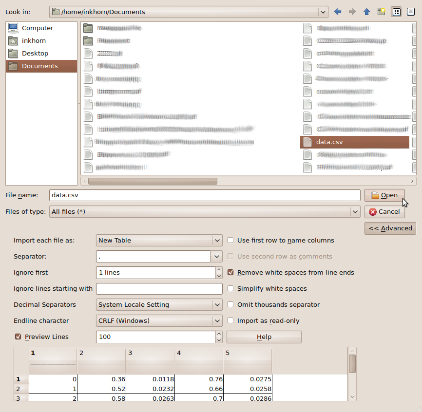
You then choose your data to import, specify the separator, whether or not you want to ignore lines at the top, then press OK.






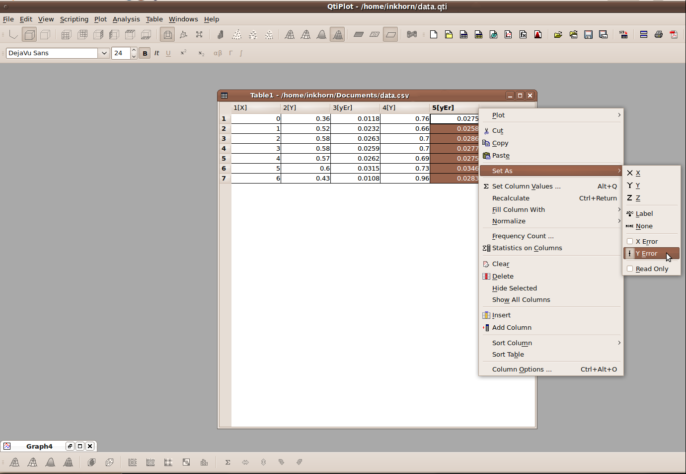
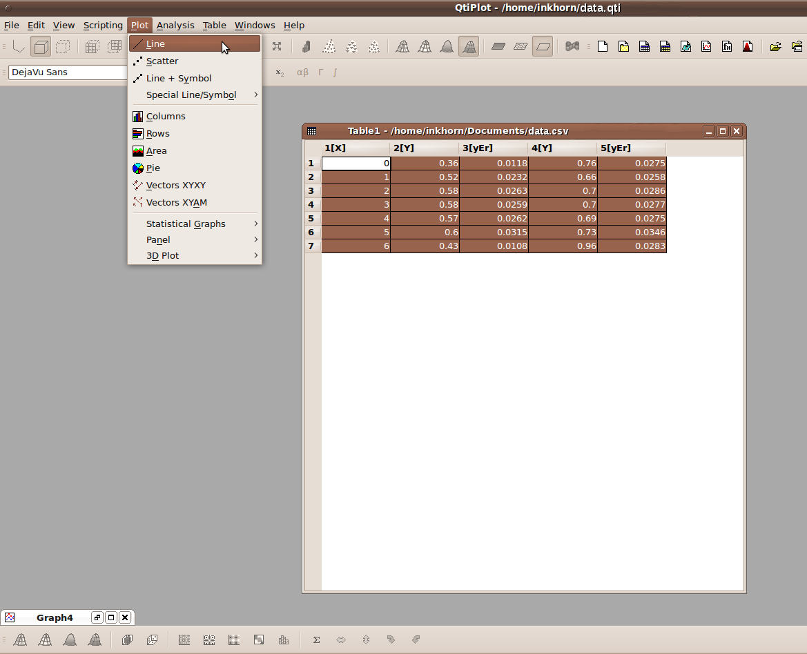
You are then shown your data in a Table view and must now right click on the columns and set their roles as shown above. As you can see, your columns can represent X variables, Y variables, Y error variables, even 3rd dimension, or Z variables. When you're done setting your column roles, navigate to the Plot menu and click on Line, as shown below.





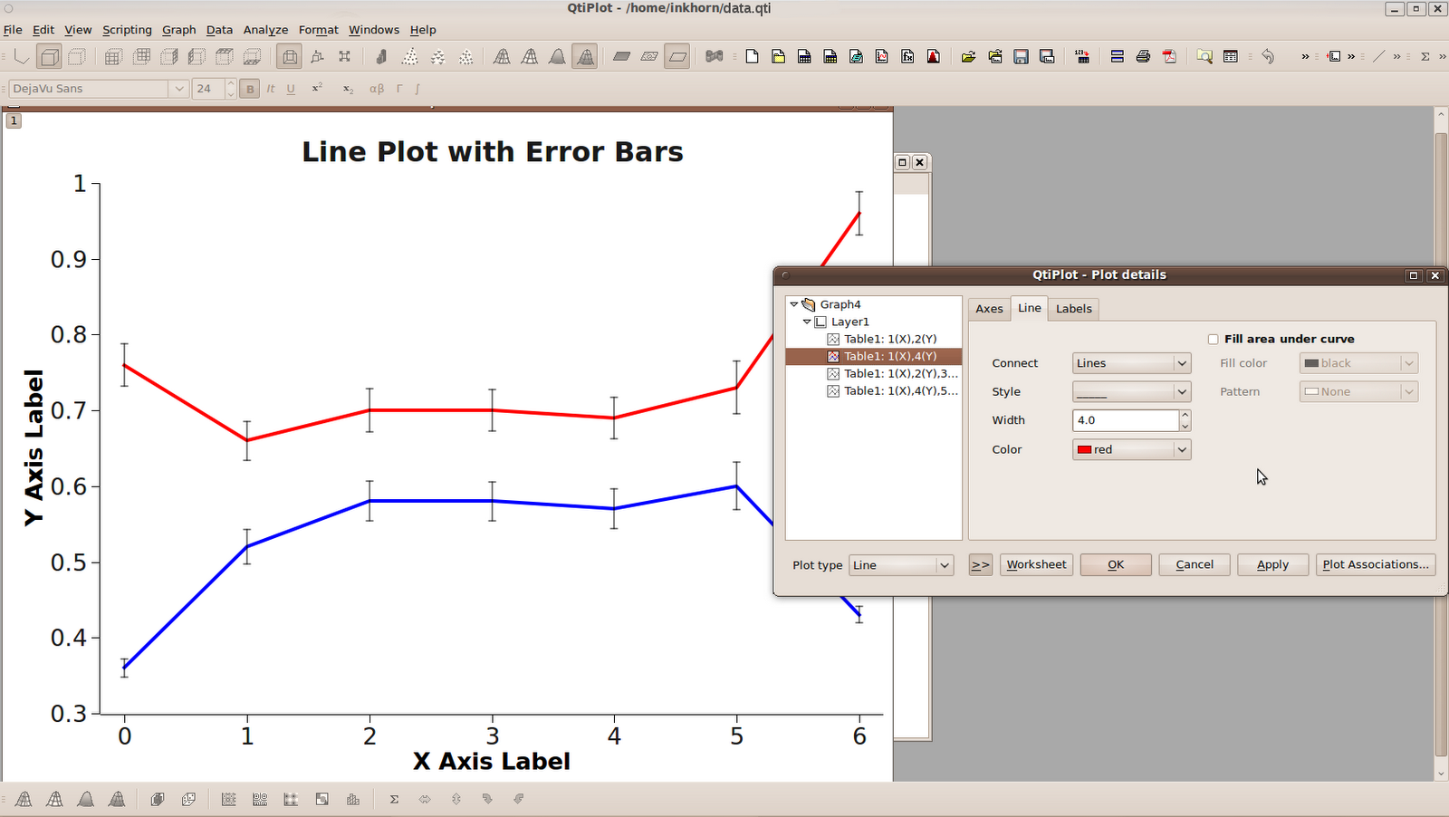
A line plot will then be generated, using default values that you can change to your heart's content. The plot title and axis titles are very easy to change; all you have to do is double click on them and edit the default text that is already there. If you want to change any other aspect of the graph, it suffices to right-click on that part of the graph, and then click on Properties, such as what I did below with one of the lines on the graph.






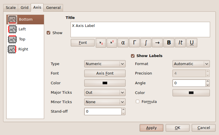
You can also modify how you want each of your axes to look by right clicking on the numbers of that axis and again clicking Properties. You can then change some general graphical properties of each axis, or change the way that the axis is scaled.



Axis options  Scale options  Once you're finished specifying your graph's visual parameters, it's then easy as pie to save it. Click File > Export Graph > Current, then choose a folder to save your graph in, name it, then press Save and you're done!



Conclusion  The truth of the matter is that you need to choose the right tool for the right job. I have often found that it was necessary for me to load data to be plotted into Ipython that I wouldn't have been able to read into R. IPython provides the opportunity for easy interactive plotting for simple one-graph projects, but can scale up to more complex programmatic plotting in larger projects. It hasn't been often that I've had to do larger scale projects where many plots are outputted programmatically, but IPython would certainly be the environment of choice for me.

R has amazingly expansive plotting capabilities and certainly does not lose points on graphical quality. As you can see however, its syntax can be difficult to manage. I've used R for making summary plots of data that I also had to statistically analyze. Therein lies the ultimate use of R; it provides a single integrated environment for the plotting and analyzing of many different types of data.

When it comes down to it, however, I am quite lazy. I only recently discovered QtiPlot, and I think it's great! According to the QtiPlot website, it even provides an interface that allows you to script QtiPlot operations using Python. I don't know anything about that interface just yet, but it makes me very impressed with the program overall. Given my laziness, the quality of the plots that come out of QtiPlot, and the ease with which you can manipulate them, QtiPlot rates very highly in my books. I will surely be using it more in the future for plotting where the data is easily accessible and will highly recommend it to others.

pyBloggerU now has a GUI

Yesterday I sat myself in front of both Qt 4 Designer and Wing IDE and didn't tear myself away from my computer until I finished a GUI for pyBloggerU.

For those who didn't read my original post on the matter, pyBloggerU is a script I made that will upload an html file containing your Blogger post and images to your Blogger account for online publication. The script deals with the weirdnesses inherent in how Blogger mangles the HTML code so that what you see in your HTML editor is not what you get on Blogger.

Unfortunately it still is not programmed to handle HTML files generated from WYSIWYG editors, as they create too many complications for me to be able to handle with this script. But I've found that creating blog posts in an HTML editor called Quanta Plus to be easy enough. Quanta Plus has lots of buttons that shoot out HTML code for you, code and tag completion, and even a Visual preview mode if you're interested.

Once you've created your blog post in an HTML editor, like Quanta Plus, you just double click on the pyBloggerU_GUI.py file, press Run at the next window and enter in all the details shown in the picture below:






Be sure that any images referred to in the HTML contain their full file paths (the one above is "/home/inkhorn/Pictures/pyBloggerU.png") so that pyBloggerU will be able to upload them from your computer to your Blog's picasa web album. When everything is set, you can press the Upload button and your HTML file will become your blog post! When pyBloggerU succeeds at sending a blog post, you'll see a "Success" information window pop up a few moments after pressing the Upload button. Also, you'll be able to save your Blogger account info by pressing Save after filling out all the fields. When you have a new post to upload to blogger, you can then double click on the entry in the list to the left and your email, password, and blog title will appear in the fields to the right.

If you would like to download pyBloggerU, it's easily acccessible as a Bazaar branch on Launchpad. Even if you don't know what a Bazaar branch on Launchpad is, go to your terminal, and type in bzr branch lp:pybloggeru. This will create a directory called pybloggeru in your home directory and will store the python files for the program and all of its dependencies therein.

Of course if you would like to report a bug, ask a question, or contribute to the program, use the web utilities on the official pyBloggerU launchpad page.

Search Workopolis Easily with Python

I've been looking for jobs lately and thought how nice it would be if I could skip the rigamarole of opening up my browser, going to a job search website, typing in the search arguments, and sifting through the results. In view of making job searching a little easier, I've made a Python script that for now will search Workopolis.com using keywords and a city location that you, the user, specify. It will then output a csv (comma separated value) file containing the job search results in the directory where you executed the script. You can then open the search results at your leisure, sift through them without the annoyances of advertisements, and possibly add them to your own database.

Just like pyBloggerU, I've uploaded the files for this Python script to launchpad for others to see and modify at their leisure. Go here if you'd like to download the program files, and here if you'd like to read more and possibly contribute to the project!

Once you put the program files in a particular directory, go to your command line, type python PyJobFinder.py, and then answer the questions that it asks you. Quickly after putting in your search terms, the program tells you the file name of the job results file and then you're free to open it up!

Blog from your HTML Editor and Python

So this is a test of the Python script I made to upload a custom made HTML file to my blog. As I mentioned in my last post, Google has provided its own Python Client Library to the public for connecting to Google's various services. What really confused me at first was the question of where exactly Google stores the pictures you want on your blog when you use the regular Blogger New Post interface. I soon discovered that if you're not linking to a picture that's on another website, any picture you put on your Blogger Blog is actually stored under a Picasa Web Album named after your blog and accessible by your Blogger account username and password. Knowing this, I just had to follow a few simple steps for using the Python Client Library to automatically upload pictures to the user's Picasa Web album (see here).

What I figured out is that if you want to put pictures on your blog post, you don't need to know where they'll be uploaded to. Just link to the pictures on your local hard drive and submit your HTML blog post file to my script. My script then:

• looks for any local image links
• uploads those files to your Picasa Web Album
• gets the URLs of your newly uploaded images
• Uses those URLs to replace the local path links in your HTML file, and finally
• Uploads your newly modified HTML file to Blogger!

Also, I noticed that Blogger ignores the header/footer html tags found in all web pages like <html>, </html>, <head>, </head>, <body>, and </body> but retains the newline codes that follow them all. Finally, when Blogger processes <br> tags that are followed by a newline code, it creates two new lines. To fix this using my script, I made it so that the inputted HTML file gets sliced from the end of the first <body> tag to just before the beginning of the </body> tag. As well, it gets rid of all <br> tags, leaving only newline codes in their places. At the moment it's a command line script that I haven't yet tested on Windows. If you'd like to take a stab at using it, download it here. To make life easy, download it to the directory where you're saving your HTML blog post file and just call it from the command line by running python pyBloggerU.py. The program will ask you for the following pieces of information:

1. The email address associated with your Blogger account
2. Your Blogger account password
3. Your Blog title (case insensitive), and finally
4. Your Blog post title

If you'd like to help me out, I've registered my project in launchpad and you can submit a branch of my code. Go here
if you want to donate your time to help me out :).

And now finally, it's time for me to test out media uploading:

Linux Blogging Solution?

I don't much like writing to this blog from the New Post interface that blogger provides.  It's too small and restricting.  So, I've done a lot of googling to find out the best way of writing to a blog from Linux.  One option I found was using Google Docs to create a text document (replete with rich text and images) and publish it to blogger.

I like the format of Google Docs and would certainly continue using it if it weren't for weird formatting incompatibilities between Google Docs and Blogger.  In other words, when writing a blog post from Google Docs and submitting it to Blogger, what you see is not exactly what you get.  I find that the text spacing and alignment become perverted when you submit a Google Docs text document to Blogger.

So, that's where the Google Data Python Library  will come in handy!  Using this set of Python modules, it's possible to upload photo media to the Picasa Web Album associated with your blog, get the associated URLs, and upload new blog posts containing your newly uploaded photos.

Using this functionality, I should be able to make a script that will take an HTML file that you create with any old web page editor, replace the links to images on your local hard drive with links to images on your picasa web album, and post your HTML file to Blogger!

Stay tuned.  I'm hoping this ends up being better than Google Docs or Scribefire (I have issues with both platforms).

Your download activity in one file!

I started downloading a very big set of files today on bittorrent (using the simple and elegant Transmission Bittorrent Client that comes with Ubuntu).  As I was watching the download speed indicator fluctuate up and down, the data analyst in me started stirring.  I thought it would be neat if I could find a program that would output my download speed over time to a dataset that I could then analyze for trends, averages, highs and lows.

I inputted the term 'bandwidth' in Synaptic Package Manager to see what kinds of programs were available for this purpose.  I found some simple command line programs such as nload, bmon, and iftop.  All of them provide text-mode screens that help you monitor your bandwidth, but none of them allow you to output download speed over time to a plain text file.

After examining the man (manual) pages for each of these programs, I noticed a commonality: each of these programs sample bandwidth information from a file named dev in the /proc/net/ directory on my computer.  Curious for more info, I navigated to that directory and opened up the file.  Here's an example of what it looks like:

If you've spent any time messing around with your network connection settings in Ubuntu (or most other operating systems) then you'll recognize most of the row titles in the above image.  Now, my computer is only connected to the net through a wireless connection to my Router/ADSL Modem.  Therefore, I don't expect any significant data in rows other than the one titled wlan0.

Next is the neat step: Linux repeatedly updates the dev file with the total number of bytes and packets received since boot-up.  All you need to do to find out the download speed in bytes/second is:

• Open the file
• Copy the numeric value just to the right of wlan0, under the bytes column
• Wait a second
• Do the same thing with the next value
• Subtract the two!

Of course nobody in their right minds would want to do this manually, but the implementation of the above algorithm is very simple in Python:

def get_bytes():
    dev = open('/proc/net/dev','rb').read()
    import re
    pat = re.compile('wlan0:\s*([0-9]+)\s*')
    return int(pat.search(dev).group(1))

def get_kbps():
    import time
    bytes1 = get_bytes()
    time.sleep(1)
    result = round(((get_bytes() - bytes1)/1000.0),1)
    return '%3.1f' % result

The first function above simply opens the dev file and returns the numeric value beside wlan0.  The second function uses the first function to get the bytes value two times and calculates Kilobytes/second (it's a smaller number than bytes/second).

I'm now using these functions to calculate Kilobytes/second every 3 seconds for a total of 4 hours to get my dataset!  If you'd like to use these functions just remember that if you're using a wired ethernet connection, change wlan0 to eth0 and you will be able get your data.